21 The Work-Energy Theorem for a Rigid Body

The Koenig decomposition for the kinetic energy of a rigid body is: \[\begin{align} T = \frac{1}{2}m{\bf v}_C\cdot{\bf v}_C+\frac{1}{2}{\bf H}^C\cdot\bomega. \end{align}\] In this class, \(\bomega = \omega{\bf E}_z\), so \(\frac{1}{2}{\bf H}^C\cdot\bomega = \frac{1}{2}I_{zz}\omega^2\).

For fixed point rotation about \(O\), the kinetic energy simplifies to: \[\begin{align} T = \frac{1}{2}{\bf H}^O\cdot\bomega \end{align}\] which further simplifies to \(T = \frac{1}{2}I^O_{zz}\omega^2\) if \(\bomega = \omega{\bf E}_z\).

The work-energy theorem for a rigid body has two equivalent forms: \[\begin{align} \frac{dT}{dt} = {\bf F}\cdot{\bf v}_C+{\bf M}^C\cdot\bomega = \sum_{i=1}^N{\bf F}_i\cdot{\bf v}_i+{\bf M}_e\cdot\bomega. \end{align}\] Integrating from \(t_A\) to \(t_B\): \[\begin{align} T_B-T_A = W_{{\bf F},AB}+W_{{\bf M},AB} = \sum_{i=1}^N W_{{\bf F}_i,AB}+W_{{\bf M}_e,AB}, \end{align}\] where \[\begin{align} W_{{\bf F},AB} &= \int_{t_A}^{t_B}{\bf F}\cdot{\bf v}_C\,dt, & W_{{\bf M},AB} &= \int_{t_A}^{t_B}{\bf M}^C\cdot\bomega\,dt,\\ W_{{\bf F}_i,AB} &= \int_{t_A}^{t_B}{\bf F}_i\cdot{\bf v}_i\,dt, & W_{{\bf M}_e,AB} &= \int_{t_A}^{t_B}{\bf M}_e\cdot\bomega\,dt. \end{align}\] Notice: the work of a force uses the velocity of its point of application.

21.1 Koenig’s Decomposition

By definition, the kinetic energy \(T\) of a rigid body is the (continuous) sum of the kinetic energies of the differential masses composing it: \[\begin{align} T = \frac{1}{2}\int_{\mathcal{B}}{\bf v}\cdot{\bf v}\,\rho\,dv. \end{align}\] We can introduce the \({\bf v}_C\) term through \[\begin{align} \begin{split} & {\bf v} = {\bf v}_C+\bomega\times\bpi,\\ & \bpi = {\bf r}-{\bf r}_C,\\ & \bomega = \omega_x{\bf e}_x+\omega_y{\bf e}_y+\omega_z{\bf e}_z. \end{split} \end{align}\] Since \[\begin{align} {\bf v}\cdot{\bf v} = ({\bf v}_C+\bomega\times\bpi)\cdot({\bf v}_C+\bomega\times\bpi) = {\bf v}_C\cdot{\bf v}_C+{\bf v}_C\cdot(\bomega\times\bpi)+(\bomega\times\bpi)\cdot{\bf v}_C+(\bomega\times\bpi)\cdot(\bomega\times\bpi), \end{align}\] and the two middle terms are equal by commutativity of the dot product, substituting the above expressions in the kinetic energy integral, we get \[\begin{align} T = \frac{1}{2}\int_{\mathcal{B}}\lp{\bf v}_C\cdot{\bf v}_C+2{\bf v}_C\cdot(\bomega\times\bpi)+(\bomega\times\bpi)\cdot(\bomega\times\bpi)\rp dm. \end{align}\] For the first two terms in the above integral, \[\begin{align} \begin{split} & \frac{1}{2}\int_{\mathcal{B}}{\bf v}_C\cdot{\bf v}_C\,dm = \frac{{\bf v}_C\cdot{\bf v}_C}{2}\int dm = \frac{1}{2}m{\bf v}_C\cdot{\bf v}_C,\\ & \int_{\mathcal{B}}{\bf v}_C\cdot(\bomega\times\bpi)\,dm = {\bf v}_C\cdot\lp\bomega\times\int\bpi\,dm\rp = 0. \end{split} \end{align}\] Thus, \[\begin{align} T = \frac{1}{2}m{\bf v}_C\cdot{\bf v}_C+\frac{1}{2}\int_{\mathcal{B}}(\bomega\times\bpi)\cdot(\bomega\times\bpi)\,dm. \end{align}\] We can simplify \((\bomega\times\bpi)\cdot(\bomega\times\bpi)\) using the scalar triple product identity \(({\bf A}\times{\bf B})\cdot{\bf C}={\bf A}\cdot({\bf B}\times{\bf C})\) with \({\bf A}=\bomega\), \({\bf B}=\bpi\), \({\bf C}=\bomega\times\bpi\): \[\begin{align} (\bomega\times\bpi)\cdot(\bomega\times\bpi) = \bomega\cdot\lp\bpi\times(\bomega\times\bpi)\rp. \end{align}\] The inner cross product expands via the BAC-CAB identity, \({\bf a}\times({\bf b}\times{\bf c}) = {\bf b}({\bf a}\cdot{\bf c})-{\bf c}({\bf a}\cdot{\bf b})\), with \({\bf a}=\bpi,{\bf b}=\bomega,{\bf c}=\bpi\): \[\begin{align} \bpi\times(\bomega\times\bpi) = (\bpi\cdot\bpi)\bomega-(\bpi\cdot\bomega)\bpi. \end{align}\] Recall that \[\begin{align} {\bf H}^C = \int_{\mathcal{B}}\bpi\times(\bomega\times\bpi)\,dm = \int_{\mathcal{B}}\lp(\bpi\cdot\bpi)\bomega-(\bpi\cdot\bomega)\bpi\rp dm. \end{align}\] Putting the last two results together, and pulling \(\bomega\) out of the integral since it is the same for every material point of the rigid body: \[\begin{align} \frac{1}{2}\int_{\mathcal{B}}(\bomega\times\bpi)\cdot(\bomega\times\bpi)\,dm = \frac{1}{2}\bomega\cdot\int_{\mathcal{B}}\bpi\times(\bomega\times\bpi)\,dm = \frac{1}{2}\bomega\cdot{\bf H}^C = \frac{1}{2}{\bf H}^C\cdot\bomega. \end{align}\] Hence, we obtain the Koenig decomposition: \[\begin{align} T = \frac{1}{2}m{\bf v}_C\cdot{\bf v}_C+\frac{1}{2}{\bf H}^C\cdot\bomega. \end{align}\]

21.1.1 Fixed Point Rotation

In the case of fixed point rotation, \({\bf v}_C = \bomega\times({\bf r}_C-{\bf r}_O)\) and \({\bf v}_O = {\bf 0}\). Since \({\bf G}=m{\bf v}_C\) is the linear momentum, \[\begin{align} \frac{1}{2}m{\bf v}_C\cdot{\bf v}_C = \frac{1}{2}(m{\bf v}_C)\cdot{\bf v}_C = \frac{1}{2}{\bf G}\cdot{\bf v}_C = \frac{1}{2}{\bf G}\cdot(\bomega\times{\bf r}_{C/O}), \end{align}\] so, using the cyclical property of the scalar triple product, \({\bf a}\cdot({\bf b}\times{\bf c}) = {\bf b}\cdot({\bf c}\times{\bf a}) = {\bf c}\cdot({\bf a}\times{\bf b})\): \[\begin{align} \begin{split} T &= \frac{1}{2}{\bf G}\cdot(\bomega\times{\bf r}_{C/O})+\frac{1}{2}{\bf H}^C\cdot\bomega\\ &= \frac{1}{2}\bomega\cdot({\bf r}_{C/O}\times{\bf G})+\frac{1}{2}{\bf H}^C\cdot\bomega\\ &= \frac{1}{2}({\bf r}_{C/O}\times{\bf G}+{\bf H}^C)\cdot\bomega\\ &= \frac{1}{2}{\bf H}^O\cdot\bomega, \end{split} \end{align}\] where the second line follows from the cyclical identity, the third line factors \(\bomega\) out of the sum of two dot products, and the last line uses the identity \[\begin{align} {\bf H}^O = {\bf H}^C+{\bf r}_{C/O}\times{\bf G}, \end{align}\] obtained by writing \[\begin{align} {\bf H}^O=\int_{\mathcal{B}}({\bf r}-{\bf r}_O)\times{\bf v}\,dm=\int_{\mathcal{B}}(\bpi+{\bf r}_{C/O})\times{\bf v}\,dm=\int_{\mathcal{B}}\bpi\times{\bf v}\,dm+{\bf r}_{C/O}\times\int_{\mathcal{B}}{\bf v}\,dm, \end{align}\] and noting that \(\int_{\mathcal{B}}\bpi\times{\bf v}\,dm={\bf H}^C\) (by the same steps used above, since \(\int\bpi\,dm={\bf 0}\)) while \(\int_{\mathcal{B}}{\bf v}\,dm=m{\bf v}_C={\bf G}\).

21.2 Derivation of the Work-Energy Theorem

Taking the time derivative of \(T = \frac{1}{2}m{\bf v}_C\cdot{\bf v}_C+\frac{1}{2}{\bf H}^C\cdot\bomega\): \[\begin{align} \dot{T} = \frac{1}{2}m\dot{\bf v}_C\cdot{\bf v}_C+\frac{1}{2}m{\bf v}_C\cdot\dot{\bf v}_C+\frac{1}{2}\dot{\bf H}^C\cdot\bomega+\frac{1}{2}{\bf H}^C\cdot\dot{\bomega}. \end{align}\] We need to show that \(\dot{\bf H}^C\cdot\bomega = {\bf H}^C\cdot\dot{\bomega}\). \[\begin{align} \begin{split} \balpha = \dot{\bomega} &= \frac{d}{dt}(\omega_x{\bf e}_x+\omega_y{\bf e}_y+\omega_z{\bf e}_z)\\ &= \dot{\omega}_x{\bf e}_x+\dot{\omega}_y{\bf e}_y+\dot{\omega}_z{\bf e}_z+\omega_x\dot{\bf e}_x+\omega_y\dot{\bf e}_y+\omega_z\dot{\bf e}_z\\ &= \dot{\omega}_x{\bf e}_x+\dot{\omega}_y{\bf e}_y+\dot{\omega}_z{\bf e}_z+\bomega\times(\omega_x{\bf e}_x+\omega_y{\bf e}_y+\omega_z{\bf e}_z)\\ &= \dot{\omega}_x{\bf e}_x+\dot{\omega}_y{\bf e}_y+\dot{\omega}_z{\bf e}_z. \end{split} \end{align}\] A direct calculation using this expression for \(\balpha\) shows that \[\begin{align} {\bf H}^C\cdot\dot{\bomega} = (I_{xx}\omega_x+I_{xy}\omega_y+I_{xz}\omega_z)\dot{\omega}_x+(I_{xy}\omega_x+I_{yy}\omega_y+I_{yz}\omega_z)\dot{\omega}_y+(I_{xz}\omega_x+I_{yz}\omega_y+I_{zz}\omega_z)\dot{\omega}_z. \end{align}\] To compute the corresponding expression for \(\dot{\bf H}^C\cdot\bomega\), recall \(\dot{\bf H}^C=\overset{\circ}{{\bf H}^C}+\bomega\times{\bf H}^C\), so \[\begin{align} \dot{\bf H}^C\cdot\bomega = \overset{\circ}{{\bf H}^C}\cdot\bomega+(\bomega\times{\bf H}^C)\cdot\bomega = \overset{\circ}{{\bf H}^C}\cdot\bomega, \end{align}\] since \((\bomega\times{\bf H}^C)\cdot\bomega=0\) (the vector \(\bomega\times{\bf H}^C\) is perpendicular to \(\bomega\)). Using the component expression for \(\overset{\circ}{{\bf H}^C}\) and dotting with \(\bomega\): \[\begin{align} \overset{\circ}{{\bf H}^C}\cdot\bomega = (I_{xx}\dot{\omega}_x+I_{xy}\dot{\omega}_y+I_{xz}\dot{\omega}_z)\omega_x+(I_{xy}\dot{\omega}_x+I_{yy}\dot{\omega}_y+I_{yz}\dot{\omega}_z)\omega_y+(I_{xz}\dot{\omega}_x+I_{yz}\dot{\omega}_y+I_{zz}\dot{\omega}_z)\omega_z. \end{align}\] Comparing this term by term with the expression for \({\bf H}^C\cdot\dot{\bomega}\) above, and using the symmetry of the inertia tensor (\(I_{xy}=I_{yx}\), \(I_{xz}=I_{zx}\), \(I_{yz}=I_{zy}\)), every term matches (e.g. \(I_{xy}\dot{\omega}_x\omega_y = I_{xy}\omega_x\dot{\omega}_y\)). Hence \(\dot{\bf H}^C\cdot\bomega = {\bf H}^C\cdot\dot{\bomega}\). Consequently, \[\begin{align} \dot{T} = \frac{1}{2}m\dot{\bf v}_C\cdot{\bf v}_C+\frac{1}{2}m{\bf v}_C\cdot\dot{\bf v}_C+\frac{1}{2}\dot{\bf H}^C\cdot\bomega+\frac{1}{2}\dot{\bf H}^C\cdot\bomega, \end{align}\] which implies that \[\begin{align} \dot{T} = m\dot{\bf v}_C\cdot{\bf v}_C+\dot{\bf H}^C\cdot\bomega. \end{align}\] Invoking the balance of linear momentum and the balance of angular momentum, we obtain the work-energy theorem: \[\begin{align} \dot{T} = {\bf F}\cdot{\bf v}_C+{\bf M}^C\cdot\bomega. \end{align}\] This is a natural extension of the work-energy theorem for a single particle.

21.3 Alternative Form

Recall, \[\begin{align} \begin{split} & {\bf F} = \sum_{i=1}^K{\bf F}_i\\ & {\bf M}^C = {\bf M}_e+\sum_{i=1}^K({\bf r}_i-{\bf r}_C)\times{\bf F}_i \end{split} \end{align}\] Hence, the mechanical power of the resultant forces and moments can be written as \[\begin{align} {\bf F}\cdot{\bf v}_C+{\bf M}^C\cdot\bomega = \lp\sum_{i=1}^K{\bf F}_i\rp\cdot{\bf v}_C+{\bf M}_e\cdot\bomega+\lp\sum_{i=1}^K({\bf r}_i-{\bf r}_C)\times{\bf F}_i\rp\cdot\bomega. \end{align}\] With \({\bf a}=\bomega\), \({\bf b}={\bf r}_i-{\bf r}_C\), \({\bf c}={\bf F}_i\), the identity \({\bf a}\cdot({\bf b}\times{\bf c}) = {\bf c}\cdot({\bf a}\times{\bf b})\) gives \[\begin{align} \lp({\bf r}_i-{\bf r}_C)\times{\bf F}_i\rp\cdot\bomega = \bomega\cdot\lp({\bf r}_i-{\bf r}_C)\times{\bf F}_i\rp = {\bf F}_i\cdot\lp\bomega\times({\bf r}_i-{\bf r}_C)\rp. \end{align}\] Substituting this into the expression for \({\bf F}\cdot{\bf v}_C+{\bf M}^C\cdot\bomega\) above: \[\begin{align} {\bf F}\cdot{\bf v}_C+{\bf M}^C\cdot\bomega = \sum_{i=1}^K{\bf F}_i\cdot{\bf v}_C+{\bf M}_e\cdot\bomega+\sum_{i=1}^K{\bf F}_i\cdot\lp\bomega\times({\bf r}_i-{\bf r}_C)\rp = \sum_{i=1}^K{\bf F}_i\cdot\lp{\bf v}_C+\bomega\times({\bf r}_i-{\bf r}_C)\rp+{\bf M}_e\cdot\bomega. \end{align}\] Noting that \({\bf v}_i = {\bf v}_C+\bomega\times({\bf r}_i-{\bf r}_C)\), we find that \[\begin{align} {\bf F}\cdot{\bf v}_C+{\bf M}^C\cdot\bomega = \sum_{i=1}^K{\bf F}_i\cdot{\bf v}_i+{\bf M}_e\cdot\bomega. \end{align}\] In conclusion, we have an alternative form of the work-energy theorem that proves to be far easier to use in applications: \[\begin{align} \dot{T} = \sum_{i=1}^K{\bf F}_i\cdot{\bf v}_i+{\bf M}_e\cdot\bomega. \end{align}\] Each force is dotted with the velocity of its point of application.

21.4 Conservative Moments

21.4.1 Torsional Spring

A torsional spring is just a model for some kind of elasticity at the joint.

A torsional spring with stiffness \(K\) creates a couple \({\bf M}_S = -K\theta{\bf E}_z\). Its power is: \[\begin{align} {\bf M}_S\cdot\bomega = -K\theta\dot{\theta} = -\frac{d}{dt}\lp\frac{K\theta^2}{2}\rp. \end{align}\] Hence \(U = \frac{1}{2}K\theta^2\) for the torsional spring.

21.4.2 Constant Couple

A constant couple \({\bf M}_e = M_e{\bf E}_z\) has power \({\bf M}_e\cdot\bomega = M_e\dot{\theta} = -\frac{d}{dt}(-M_e\theta)\). Hence \(U = -M_e\theta\).

Note!

These results apply only for \(\bomega = \omega{\bf E}_z\). Constant couples are not conservative in general.

21.5 Examples

21.5.1 Bar Pendulum Fixed at Its End

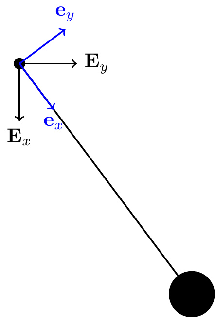
A bar of length \(\ell\) and mass \(m\) pinned at its end. The energy is conserved: \[\begin{align} U &= -\frac{mg\ell}{2}\cos\theta,\\ E &= \frac{m\ell^2}{6}\dot{\theta}^2-\frac{mg\ell}{2}\cos\theta = \text{const}. \end{align}\]

21.5.2 Bar Pendulum With End Mass

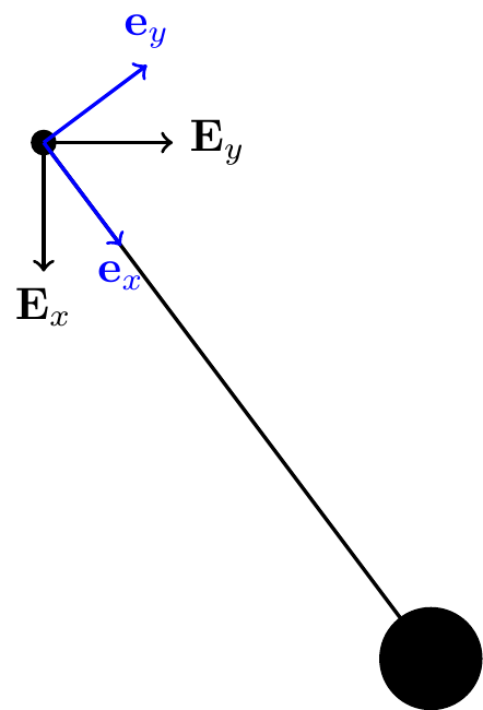
Adding a dead mass \(m_e\) at the end: \[\begin{align} U = -\frac{mg\ell}{2}\cos\theta-m_e g\ell\cos\theta. \end{align}\]

21.5.3 Follower Force

What happens if there is a follower force applied at the end of the rod always perpendicular to it?

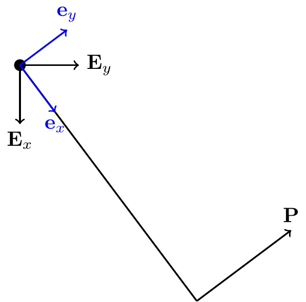
If instead a follower force \({\bf P}\) is applied perpendicular to the bar at its end, this force is nonconservative (its direction actively changes with configuration). Energy is not conserved.

21.6 Energy Conservation

As with particles and systems of particles, this theorem can be used to establish conservation of the total mechanical energy of a rigid body, \(E = T + U\), when all work-doing forces and moments are conservative.

21.7 Summary

Koenig decomposition of kinetic energy: \[\begin{align} T = \tfrac{1}{2}m\mathbf{v}_C\cdot\mathbf{v}_C + \tfrac{1}{2}\mathbf{H}^C\cdot\boldsymbol{\omega}. \end{align}\] If a point \(O\) has zero velocity: \(T = \tfrac{1}{2}\mathbf{H}^O\cdot\boldsymbol{\omega}\).

Work–energy theorem for a rigid body: \[\begin{align} \frac{dT}{dt} = \mathbf{F}\cdot\mathbf{v}_C + \mathbf{M}\cdot\boldsymbol{\omega} = \sum_i \mathbf{F}_i\cdot\mathbf{v}_i + M_e\omega. \end{align}\]

21.8 Exercises

The following problems are from Set 23 – Work–Energy Theorem for Rigid Bodies.

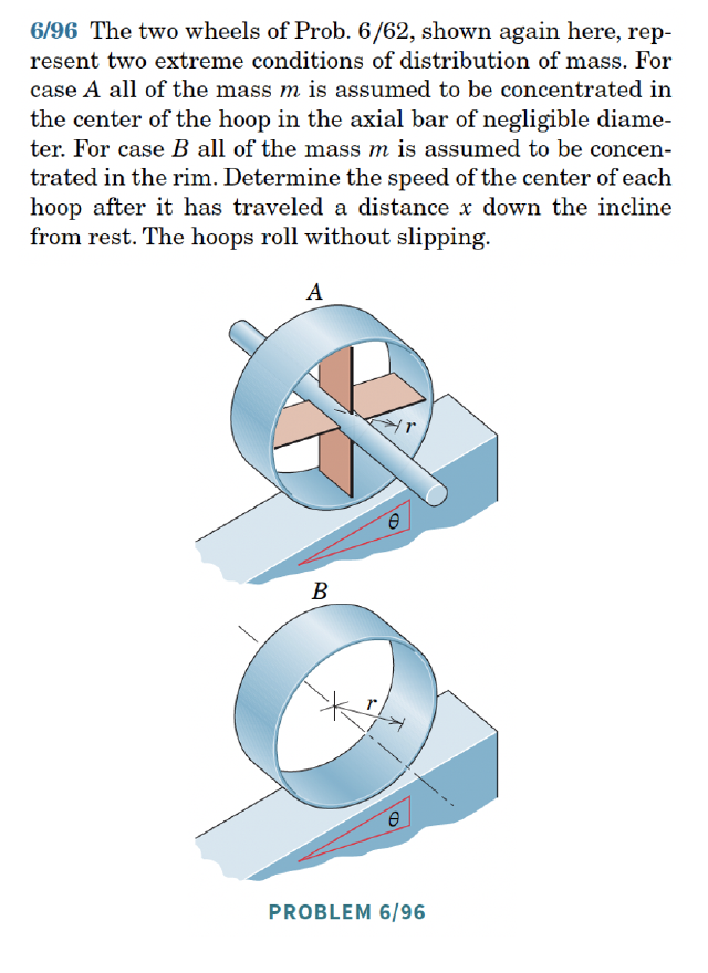
1. [MKB 06-096] (ans. \(v_A=\sqrt{2gx\sin\theta}\), \(v_B=\sqrt{gx\sin\theta}\))

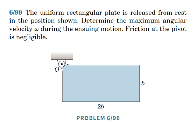
2. [MKB 06-099] (ans. \(\omega_{\max}=0.861\sqrt{g/b}\))

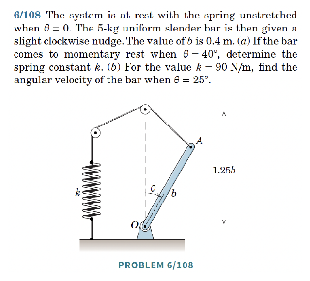
3. [06-108] (ans. (a) \(k=93.3\) N/m; (b) \(\omega=1.484\) rad/s CW)

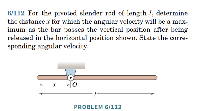
4. [06-112] (ans. \(x=0.211l\), \(\omega_{\max}=1.861\sqrt{g/l}\) CW)

5. [06-118] (ans. \(v_A=\sqrt{3}\sqrt{\frac{M\theta}{m}-gb(1-\cos\theta)}\) right)