20 Kinetics of Rigid Bodies

20.1 Balance Laws for a Rigid Body

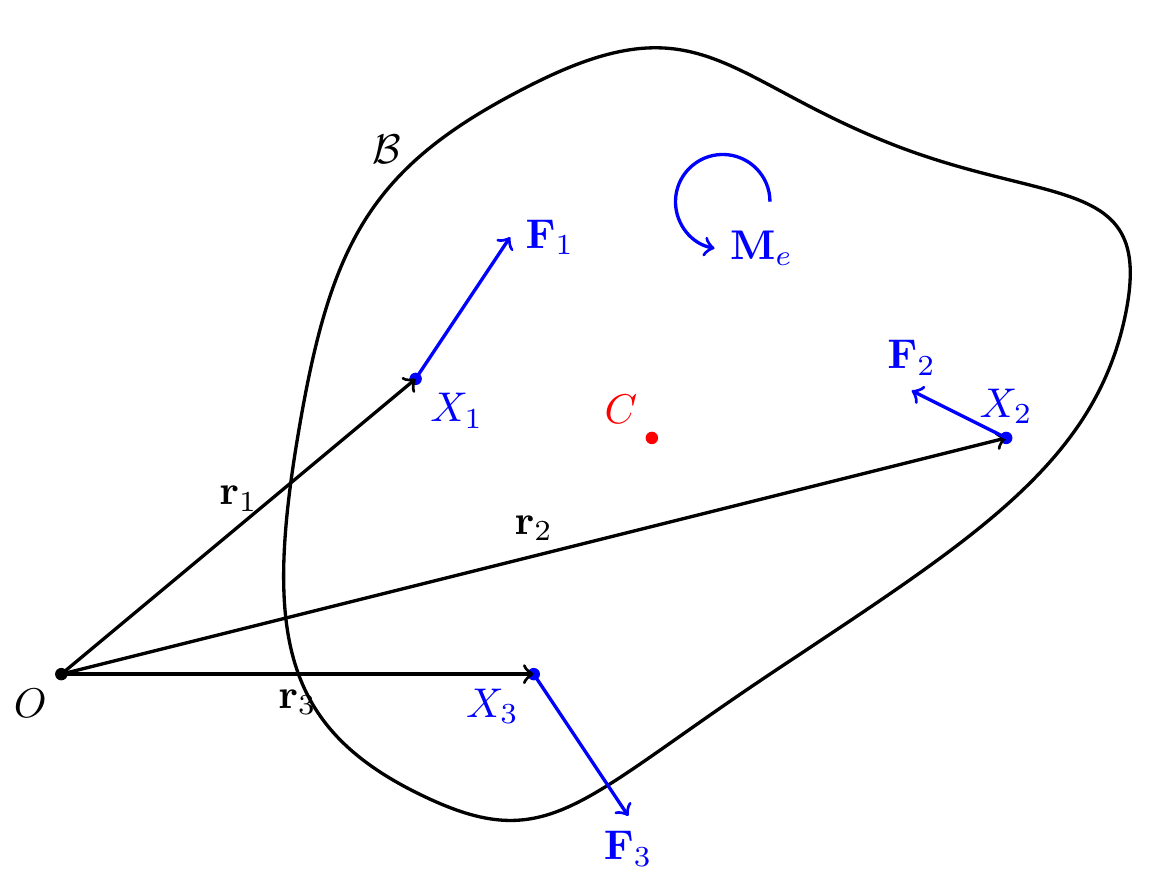
The balance laws for a rigid body are Euler’s first law (Balance of Linear Momentum, BoLM) \[\begin{align} {\bf F} &= m{\bf a}_C, \end{align}\] and Euler’s second law (Balance of Angular Momentum, BoAM), which can be expressed in three equivalent forms: \[\begin{align} {\bf M}^O &= \dot{\bf H}^O \quad\text{about a fixed point }O,\\ {\bf M}^C &= \dot{\bf H}^C \quad\text{about the center of mass }C,\\ {\bf M}^P &= \dot{\bf H}^P+({\bf v}_P-{\bf v}_C)\times{\bf G} = \dot{\bf H}^C+({\bf r}_C-{\bf r}_P)\times m{\bf a}_C \quad\text{about any material point }P. \end{align}\] The BoAM is an independent postulate, not derivable from the BoLM.

Historical Perspective: Leonhard Euler (1707–1783)

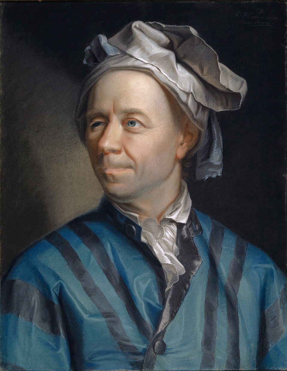
Portrait by Emanuel Handmann, 1753 (Wikimedia Commons, public domain).

Swiss mathematician and physicist, one of the most prolific scientists in history. Euler recast Newton’s mechanics in the vectorial, differential-equation form used today, and in 1750 he was the first to state the balance of linear and angular momentum as independent postulates for a general body – the two balance laws that bear his name above.

Historical Perspective: Euler’s Original Paper (1750)

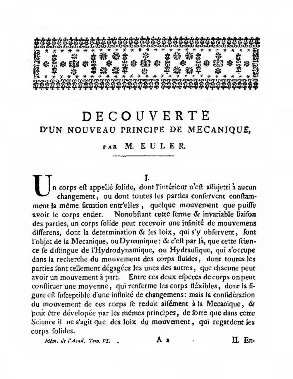
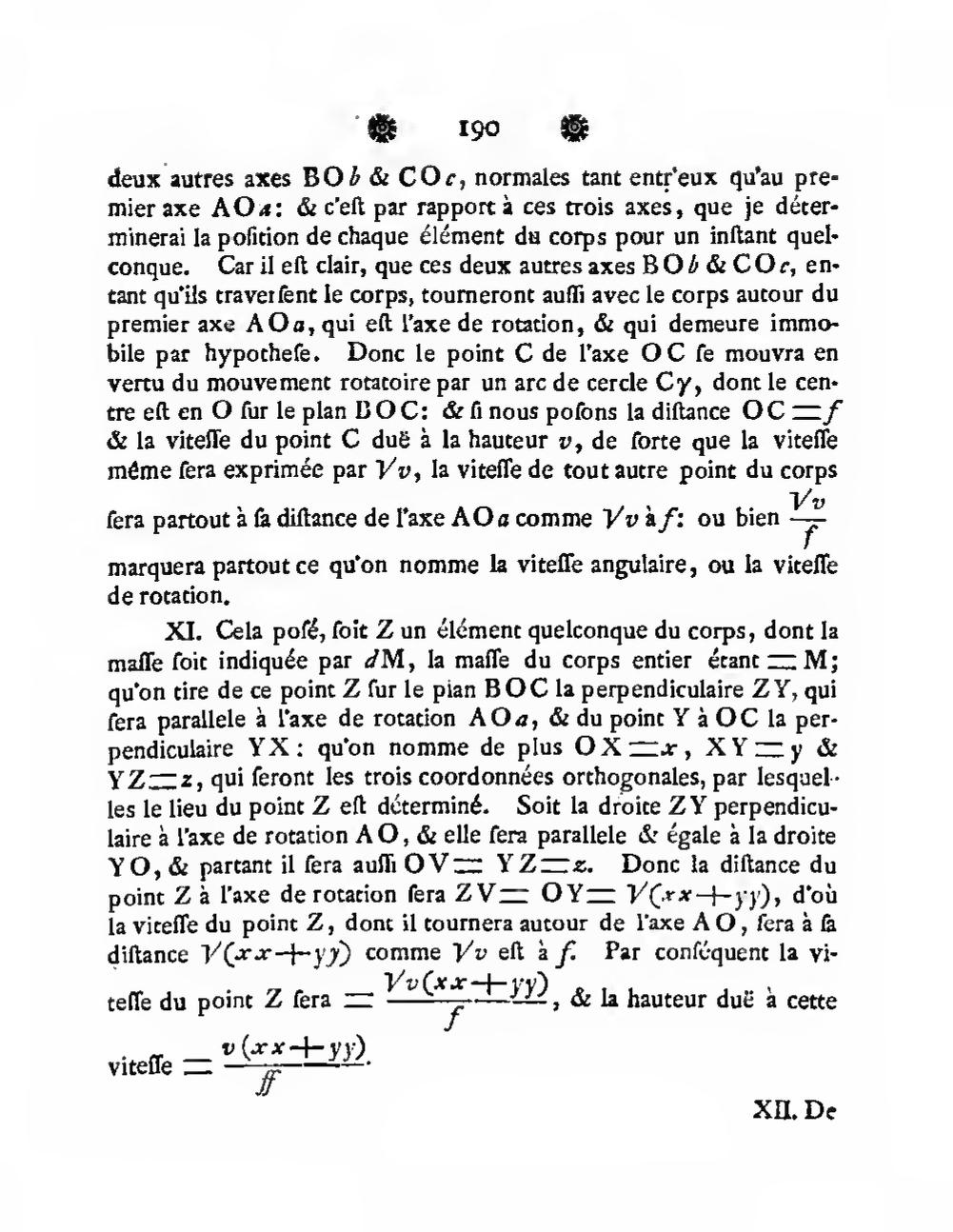
Opening page (archive.org, public domain).

The page stating the balance laws (archive.org, public domain).

Euler’s “Découverte d’un nouveau principe de mécanique,” Mémoires de l’Académie des sciences de Berlin, 1750. In this paper, Euler proposed that ${\bf F}=m{\bf a}$ (his “first law”) should be applied not only to particles, as Newton had done, but independently to every infinitesimal element of a body, and introduced the balance of angular momentum (his “second law”) as a separate, independent postulate – the foundation of rigid body dynamics used in this chapter.

20.2 Resultant Forces and Moments

The resultant force ${\bf F}$ is the sum of all external forces. The resultant moment about a point includes the moment due to forces plus any applied pure moments ${\bf M}_e$ not due to forces.

For $K$ forces ${\bf F}_i$ acting at positions ${\bf r}_i$ plus a pure moment ${\bf M}_e$: \[\begin{align} {\bf F} &= \sum_{i=1}^K{\bf F}_i,\\ {\bf M}^O &= {\bf M}_e+\sum_{i=1}^K{\bf r}_i\times{\bf F}_i,\\ {\bf M}^C &= {\bf M}_e+\sum_{i=1}^K({\bf r}_i-{\bf r}_C)\times{\bf F}_i. \end{align}\]

Examples of pure moments: reaction moments ${\bf M}_R$ at joints; torsional spring moments $-K_T(\theta-\theta_0){\bf E}_z$.

20.2.1 Does Weight Result in a Moment About the Center of Mass?

The total weight is ${\bf W} = \int_{\mathcal{B}}{\bf g}\,dm = {\bf g}\int_{\mathcal{B}}dm = m{\bf g}$, and its moment about $C$ is: \[\begin{align} {\bf M}^C = \int_{\mathcal{B}}\bpi\times{\bf g}\,dm = \lp\int_{\mathcal{B}}\bpi\,dm\rp\times{\bf g} = {\bf 0}, \end{align}\] since $\int_{\mathcal{B}}\bpi\,dm = {\bf 0}$ by definition of the center of mass.

20.3 Equivalence of the BoAM Forms

The following devepments are true for rigid bodies where the inertia matrix is constant in the body frame.

20.3.1 BoAM About Any Point $P$

Starting from ${\bf M}^C = \dot{\bf H}^C$ and replacing ${\bf M}^P = {\bf M}^C+({\bf r}_C-{\bf r}_P)\times{\bf F}$: \[\begin{align} {\bf M}^P = \dot{\bf H}^C+({\bf r}_C-{\bf r}_P)\times{\bf F}. \end{align}\] Substituting $\dot{\bf H}^C = \dot{\bf H}^P+({\bf v}_P-{\bf v}_C)\times{\bf G}+({\bf r}_P-{\bf r}_C)\times m{\bf a}_C$ and simplifying: \[\begin{align} \begin{split} {\bf M}^P &= \dot{\bf H}^P+({\bf v}_P-{\bf v}_C)\times{\bf G}+({\bf r}_P-{\bf r}_C)\times m{\bf a}_C+({\bf r}_C-{\bf r}_P)\times{\bf F},\\ &= \dot{\bf H}^P+({\bf v}_P-{\bf v}_C)\times{\bf G}, \end{split} \end{align}\] recovering the BoAM about a general material point $P$.

20.3.2 BoAM About a Fixed Point $O$

If $P$ is a fixed point $O$ (so ${\bf v}_O = {\bf 0}$), the above simplifies to ${\bf M}^O = \dot{\bf H}^O$.

Think!

Question: When is the angular momentum of a rigid body about a fixed point $O$ or about its center of mass $C$ conserved? Under what conditions are these anguar momenta conserved in a certain direction (eg. along ${\bf E}_z$)?

Answer

20.4 Calculating the Derivative of Angular Momentum

Recall that \[\begin{align} \begin{split} {\bf H}^P = {\bf I}^P\bomega+({\bf r}_C-{\bf r}_P)\times m{\bf v}_P \end{split} \end{align}\] if $P$ is taken to be the center of mass $C$ or a fixed point $O$ respectively, we get \[\begin{align} \begin{split} {\bf H}^C = {\bf I}^C\bomega,\\ {\bf H}^P = {\bf I}^P\bomega. \end{split} \end{align}\] In component form, \[\begin{align} {\bf H}^C = (I_{xx}^C\omega_x+I_{xy}^C\omega_y+I_{xz}^C\omega_z){\bf e}_x+(I_{xy}^C\omega_x+I_{yy}^C\omega_y+I_{yz}^C\omega_z){\bf e}_y+(I_{xz}^C\omega_x+I_{yz}^C\omega_y+I_{zz}^C\omega_z){\bf e}_z. \end{align}\] where \[\begin{align} \bomega = \omega_x{\bf e}_x+\omega_y{\bf e}_y+\omega_z{\bf e}_z. \end{align}\] We need to calculate $\dot{\bf H}^C$. \[\begin{align} \dot{\bf H}^C=\overset{\circ}{{\bf H}^C}+\bomega\times{\bf H}^C. \end{align}\] where $\overset{\circ}{{\bf H}^C}$ is the corotational rate of ${\bf H}$, that is the time derivative of ${\bf H}$ that is obtained while keeping ${\bf e}_x$, ${\bf e}_y$, and ${\bf e}_z$ fixed: \[\begin{align} \overset{\circ}{{\bf H}^C} = (I_{xx}^C\dot{\omega}_x+I_{xy}^C\dot{\omega}_y+I_{xz}^C\dot{\omega}_z){\bf e}_x+(I_{xy}^C\dot{\omega}_x+I_{yy}^C\dot{\omega}_y+I_{yz}^C\dot{\omega}_z){\bf e}_y+(I_{xz}^C\dot{\omega}_x+I_{yz}^C\dot{\omega}_y+I_{zz}^C\dot{\omega}_z){\bf e}_z. \end{align}\] For the case where $\bomega=\omega{\bf E}_z$ considered exclusively in this class, the previous expressions simplify to \[\begin{align} \begin{split} {\bf H}^C &= I_{xz}^C\omega_z{\bf e}_x+I_{yz}^C\omega_z{\bf e}_y+I_{zz}^C\omega_z{\bf e}_z,\\ \dot{\bf H}^C &= (I_{xz}^C\dot{\omega}-I_{yz}^C\omega^2){\bf e}_x+(I_{yz}^C\dot{\omega}+I_{xz}^C\omega^2){\bf e}_y+I_{zz}^C\dot{\omega}{\bf E}_z. \end{split} \end{align}\] Analogous developments yield \[\begin{align} \begin{split} & \dot{\bf H}^O = (I_{xz}^O\dot{\omega}-I_{yz}^O\omega^2){\bf e}_x+(I_{yz}^O\dot{\omega}+I_{xz}^O\omega^2){\bf e}_y+I_{zz}^O\dot{\omega}{\bf E}_z,\\ & \dot{\bf H}^C = (I_{xz}^C\dot{\omega}-I_{yz}^C\omega^2){\bf e}_x+(I_{yz}^C\dot{\omega}+I_{xz}^C\omega^2){\bf e}_y+I_{zz}^C\dot{\omega}{\bf E}_z,\\ & \dot{\bf H}^P = (I_{xz}^P\dot{\omega}-I_{yz}^P\omega^2){\bf e}_x+(I_{yz}^P\dot{\omega}+I_{xz}^P\omega^2){\bf e}_y+I_{zz}^P\dot{\omega}{\bf E}_z+\frac{d}{dt}\left(({\bf r}_C-{\bf r}_P)\times m{\bf v}_P\right). \end{split} \end{align}\] For fixed axis rotation, it is generally better to sum the moments about a fixed point passing through the axis of rotation. For general plane motion, there is no fixed point, so the BoAM is either summed about the center of mass or about a general material point $P$ on the body.

Note!

Remember, the BoAM about a general point has additional terms to ${\bf I}^P\bomega$: \[\begin{align} \begin{split} {\bf M}^P &= (I_{xz}^P\dot{\omega}-I_{yz}^P\omega^2){\bf e}_x+(I_{yz}^P\dot{\omega}+I_{xz}^P\omega^2){\bf e}_y+I_{zz}^P\dot{\omega}{\bf E}_z+({\bf v}_P-{\bf v}_C)\times{\bf G},\\ &= (I_{xz}^C\dot{\omega}-I_{yz}^C\omega^2){\bf e}_x+(I_{yz}^C\dot{\omega}+I_{xz}^C\omega^2){\bf e}_y+I_{zz}^C\dot{\omega}{\bf E}_z + ({\bf r}_C-{\bf r}_P)\times m{\bf a}_C. \end{split} \end{align}\]

20.5 Impact Problems and Center of Percussion

For rigid bodies, impact ideas are the same as in systems of particles.

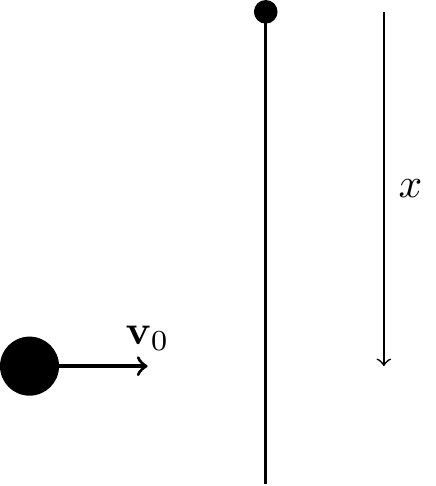
Example: Consider a projectile fired horizontally at a pendulum (in the horizontal plane, no gravity). Find position $x$ along the pendulum such that the reaction force at the pin is nearly zero during impact. If $x$ is large, the horizontal reaction at $O$ points left; if $x$ is small, it points right. The optimal $x$ that minimizes the reaction is called the center of percussion.

20.6 Impulse and Momentum for Rigid Bodies

The linear impulse - linear momentum equation is \[\begin{align} \int_{t_A}^{t^B}{\bf F}dt = {\bf G}(t_B)-{\bf G}(t_A). \end{align}\] The angular impulse - angular momentum equations are equivalently \[\begin{align} & \int_{t_A}^{t_B}{\bf M}^C dt = {\bf H}^C(t_B)-{\bf H}^C(t_A)\quad\text{where $C$ is the center of mass},\\ & \int_{t_A}^{t_B}{\bf M}^O dt = {\bf H}^O(t_B)-{\bf H}^O(t_A)\quad\text{if there is a fixed point }O. \end{align}\]

20.7 Moment-Free Motion of a Rigid Body

The Tennis Racket Problem: A tennis racket is thrown in the air with a certain angular velocity. The racket rotates about its center of mass, and the angular momentum is conserved. The racket has three principal axes of rotation, and the stability of rotation depends on which axis is used. Rotation about the axis with the largest or smallest moment of inertia is stable, while rotation about the intermediate axis is unstable.

This is also known as the Dzhanibekov effect.

You can learn more about this here and here.

https://www.youtube.com/watch?v=1VPfZ_XzisU&t=22s

20.8 Summary

For $K$ forces and a moment ${\bf M}_e$ acting on a rigid body, the balance laws are: \[\begin{align} {\bf F} = m\frac{d{\bf v}_C}{dt}, \qquad {\bf M}^O = \dot{\bf H}^O \quad (\text{or equivalently } {\bf M}^C = \dot{\bf H}^C). \end{align}\]

For fixed-axis rotation with $\bomega = \omega{\bf E}_z$ and $I_{xz}=I_{yz}=0$: \[\begin{align} {\bf F} = m\dot{\bf v}_C, \qquad {\bf M} = I_{zz}\dot{\omega}{\bf E}_z. \end{align}\]

Four classes of applications: (1) purely translational motion ($\bomega=\balpha={\bf 0}$), (2) rigid body with a fixed point, (3) rolling and sliding rigid bodies, (4) imbalanced rotors.

It is important to note that for the second set of applications, the balance law ${\bf M}^O=\dot{\bf H}^O$ is more convenient to use than ${\bf M}=\dot{\bf H}$. The role of ${\bf M}_R$ in these problems is to ensure that the axis of rotation remains ${\bf E}_z$. Finally, the four steps discussed are used as a guide to solving all of the applications.

20.9 Exercises

20.9.1 Set 19 – Rigid Body Translation

1. [MKB 06-006] (ans. $a=5.66$ m/s$^2$)

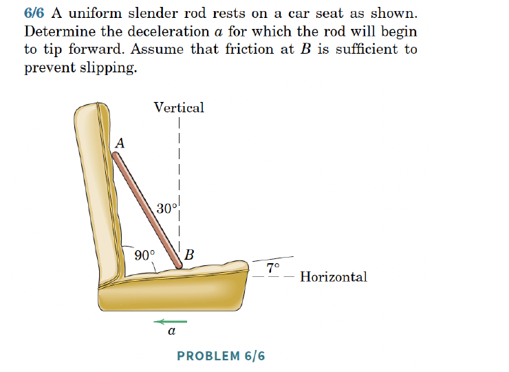
2. [06-012] (ans. $a=16.43$ ft/sec$^2$)

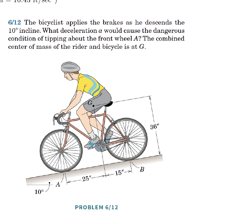
3. [06-013] (ans. $N_A=6.85$ kN up, $N_B=9.34$ kN up)

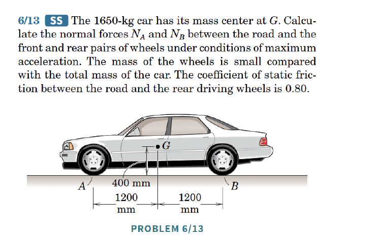
4. [06-022] (ans. $N=257$ kN up)

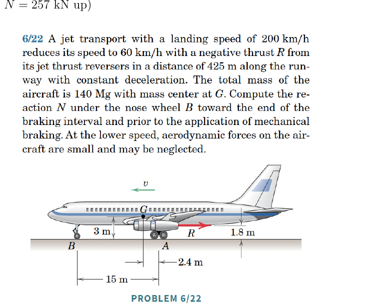
20.9.2 Set 20 – Fixed Point Rotation

1. [MKB 06-029] (ans. $\alpha=1.193$ rad/s$^2$ CCW, $F_A=769$ N)

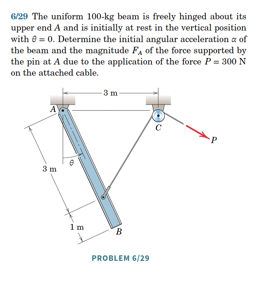
2. [MKB 06-035] (ans. $R=3.57$ lb)

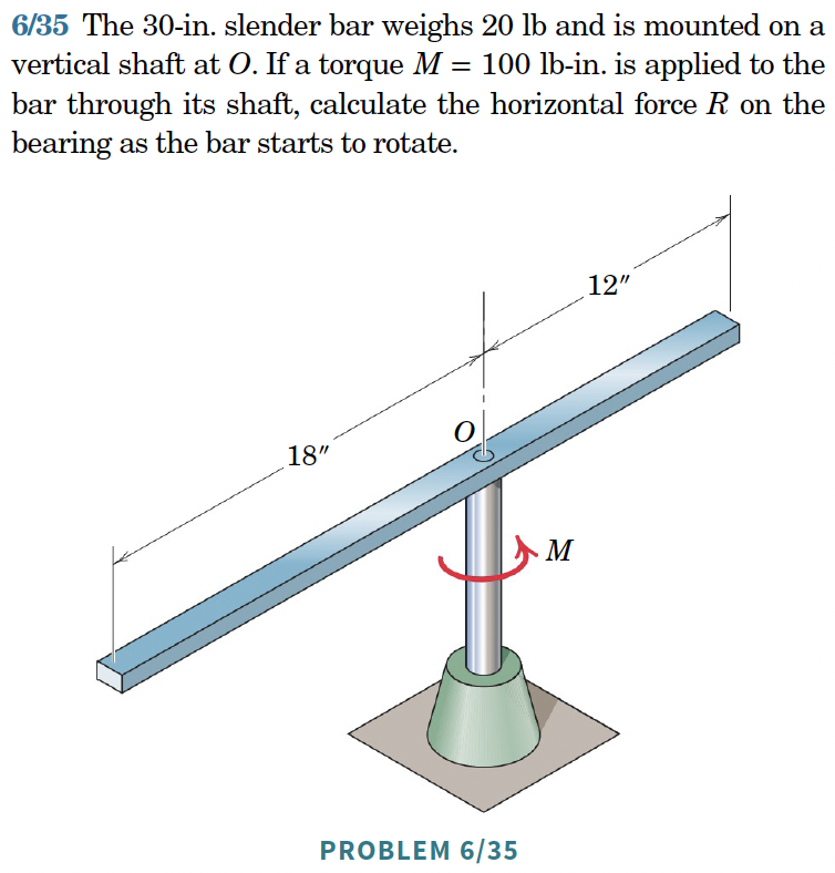
3. [06-037] (ans. $A=56.3$ N)

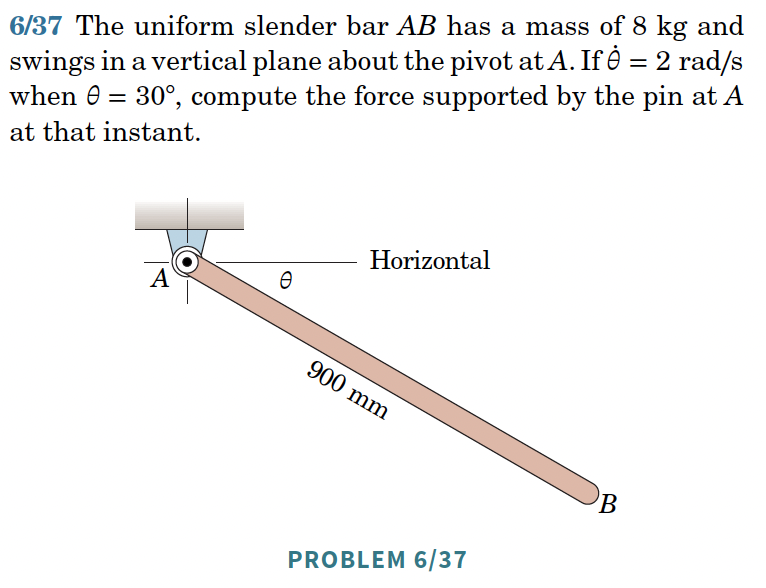
4. [06-039] (ans. (a) $\alpha=7.85$ rad/s$^2$ CCW, (b) $\alpha=6.28$ rad/s$^2$ CCW)

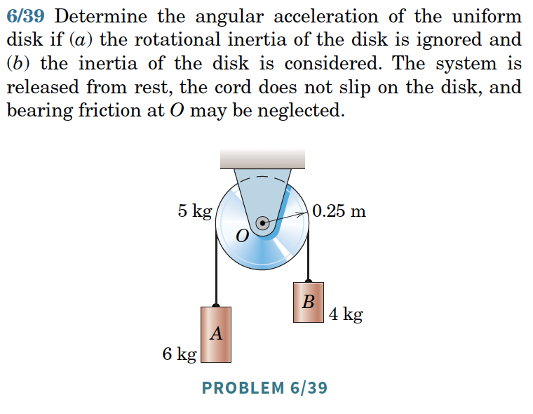
5. [06-051] (ans. $b=40.7$ mm, $R=167.8$ N)

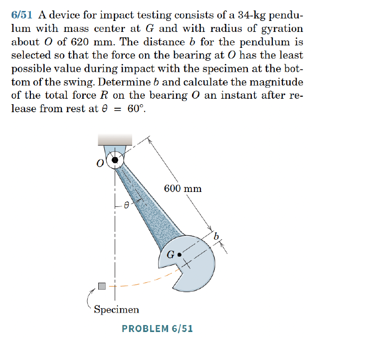
6. [06-054] (ans. $\alpha=\frac{6g}{7l}-\frac{12k}{7m}(\sqrt{5}-\sqrt{3})$)

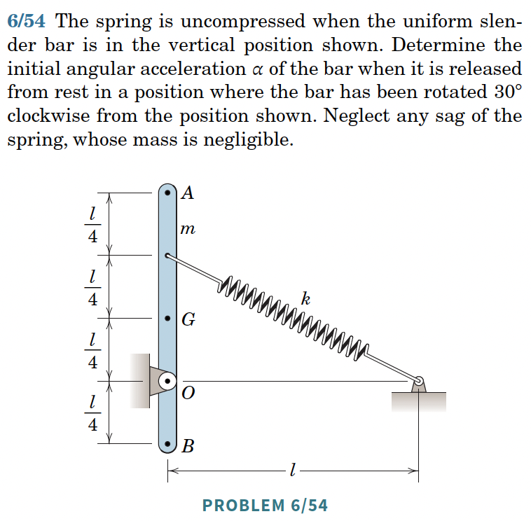
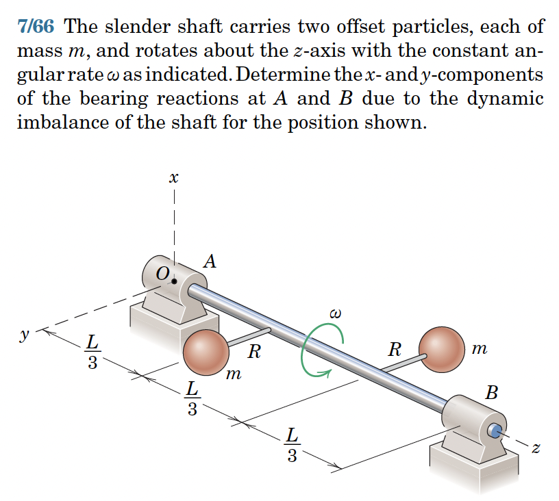
7. [MKB 07-066] Dynamic imbalance of a rotating shaft carrying two offset point masses.

20.9.3 Set 21 – General Plane Motion

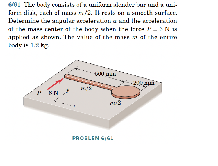
1. [MKB 06-061] (ans. $\alpha=48.8$ rad/s$^2$ CW, $\bar a_x=0$, $\bar a_y=5$ m/s$^2$)

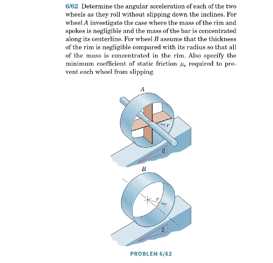
2. [MKB 06-062] (ans. A: $\alpha_A=\frac{g}{r}\sin\theta$, $\mu_s=0$; B: $\alpha_B=\frac{g}{2r}\sin\theta$, $\mu_s=\frac{1}{2}\tan\theta$)

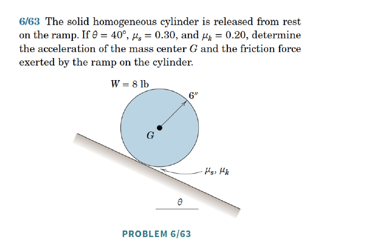
3. [06-063] (ans. $\bar a=13.80$ ft/sec$^2$ down incline, $F=1.714$ lb up incline)

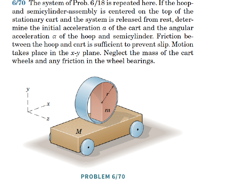
4. [06-070] (ans. $a=\frac{8(m+M)g}{3\pi(m+3M)}$ left, $\alpha=\frac{8mg}{3\pi r(m+3M)}$ CW)

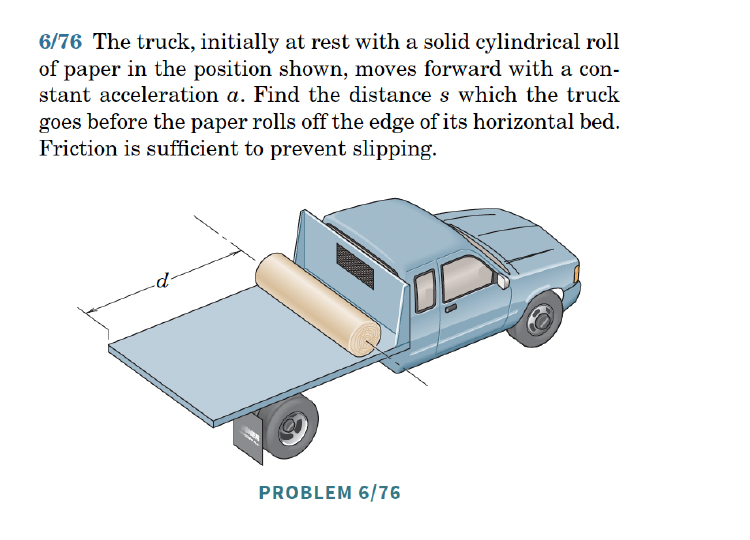
5. [06-076] (ans. $s=\frac{3d}{2}$)

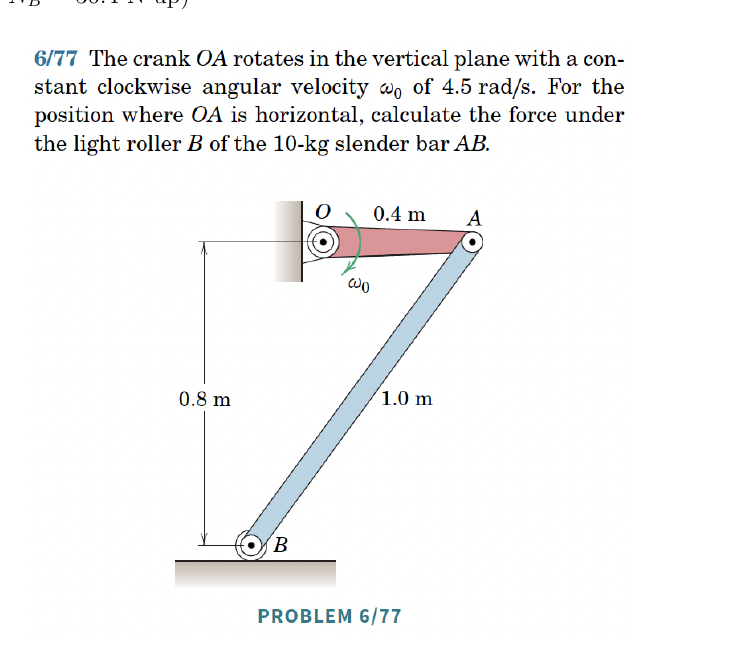
6. [06-077] (ans. $N_B=36.4$ N up)

20.9.4 Set 22 – Impulse and Momentum for Rigid Bodies

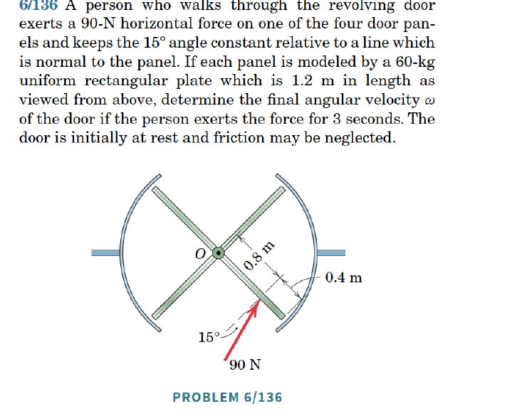
1. [MKB 06-136] (ans. $\omega=1.811$ rad/s CCW)

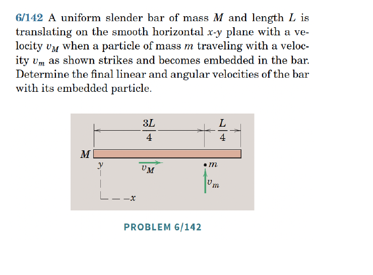
2. [MKB 06-142] (ans. $\mathbf{v}=\frac{Mu_M\mathbf{E}_x+m\mathbf{v}_m}{M+m}$, $\omega=\frac{12vm}{L(4M+7m)}$ CCW)

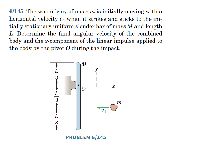
3. [06-145] (ans. $\omega=\frac{3mv_1}{(M+m)L}$ CW)

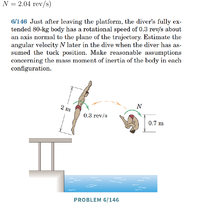
4. [06-146] (ans. $N=2.04$ rev/s)

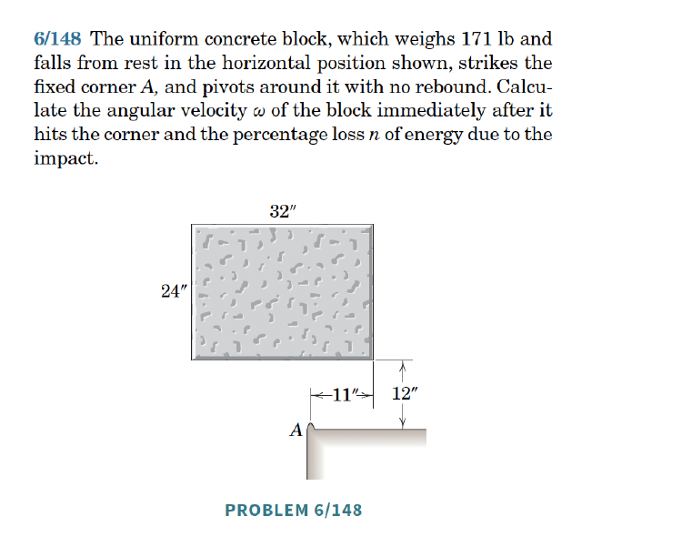
5. [06-148] (ans. $\omega=1.593$ rad/s CCW, $n=91.7\%$)

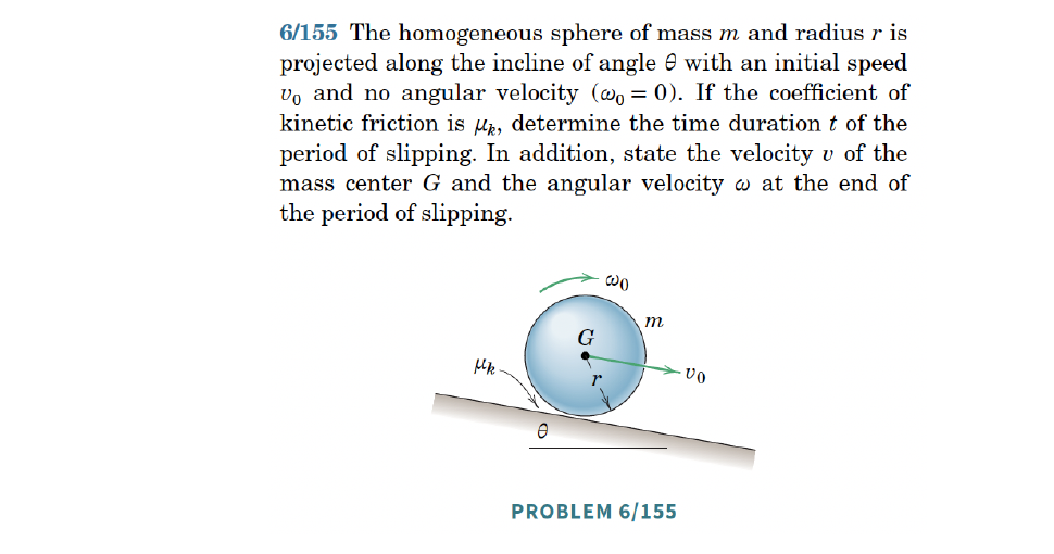
6. [06-155] (ans. $t=\frac{2v_0}{g(7\mu_k\cos\theta-2\sin\theta)}$)