8 Particle Kinetics
8.1 The Balance of Linear Momentum
A particle is endowed with an inertial measure \(m\), called its mass.
The linear momentum of a particle is defined to be \[\begin{align} {\bf G} = m{\bf v}. \end{align}\] Taking the time derivative: \[\begin{align} \dot{\bf G} = \dot{m}{\bf v}+m\dot{\bf v}. \end{align}\]
TipThink!
Question: Can you think of systems whose mass is not conserved?
NoteAnswer
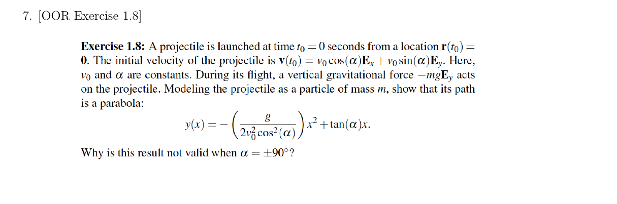
In this class, we consider cases where mass is conserved, i.e. \(\dot{m} = 0\). This is not the case, for example, for a launching rocket that is losing mass. The \(\dot{m}{\bf v}\) term is useful in control volume analysis.
Then, in our case of interest: \[\begin{align} \dot{\bf G} = m\dot{\bf v} = m{\bf a}. \end{align}\] We postulate the following balance law/axiom/postulate to be true: \[\begin{align} {\bf F} = \dot{\bf G}, \end{align}\] where \({\bf F}\) is the resultant external force acting on the particle. This is known as the Balance of Linear Momentum, Newton’s Second Law, or Euler’s First Law.
Historical Perspective: Newton’s Principia (1687)
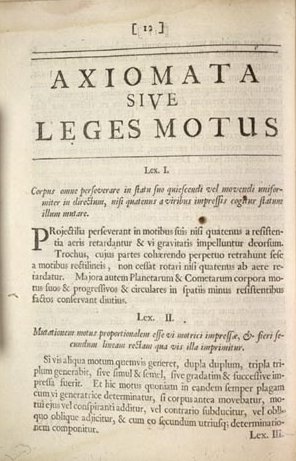
This is the page on which Newton first stated, in Latin, the three laws of motion used throughout this chapter – including the balance of linear momentum above, and Newton’s Third Law, stated later in this chapter.
Important: \({\bf a}\) here is the absolute acceleration vector of the particle.
TipThink!
Question: Under what conditions is the linear momentum \({\bf G}\) conserved?
NoteAnswer
An unbalanced net force \({\bf F}\neq {\bf 0}\) results in a change of \({\bf G}\). If \({\bf F}={\bf 0}\), then \({\bf G}={\bf c}\) where \({\bf c}\) is a constant vector. This is Newton’s First Law.
If \({\bf c}={\bf 0}\), we recover statics.
8.1.1 Representations and Projections
Vectors are represented on a basis. For example: \[\begin{align} {\bf F} &= F_x{\bf E}_x+F_y{\bf E}_y+ F_z{\bf E}_z,\\ {\bf a} &= a_x{\bf E}_x+a_y{\bf E}_y+a_z{\bf E}_z. \end{align}\]
TipThink!
Question: How many independent scalar equations can we obtain from \({\bf F}=m{\bf a}\)? How do we obtain them?
NoteAnswer
We get useful scalar equations by projecting \({\bf F} = \dot{\bf G}\) along unit directions: \[\begin{align} \lp{\bf F}=\dot{\bf G}\rp\cdot{\bf E}_x \implies F_x = ma_x. \end{align}\]
8.2 Newton’s Third Law
When dealing with the forces of interaction between particles, a particle and a rigid body, or rigid bodies, we also invoke Newton’s third law: “For every action there is an equal and opposite reaction.” For example, the force exerted by a surface on a particle is equal in magnitude and opposite in direction to the force exerted by the particle on the surface.
8.3 Four Steps to Problem Solving Using the BoLM
- Specify the system you are considering. Pick a frame (choose an origin and a coordinate system), and express \({\bf r}\), \({\bf v}\) and \({\bf a}\) using that coordinate system.
- Draw a Free Body Diagram (FBD), i.e. model of the forces.
- Write the balance of linear momentum for the system: \({\bf F}=\dot{\bf G}\).
- Do the analysis: project \({\bf F}=\dot{\bf G}\) to get useful equations.
8.3.1 Example: Projectile Motion
Projectile motion is a curvilinear motion in the plane \(\mathbb{E}^2\).
Choose \(O\) at the launch point, \({\bf E}_x\) along the ground, \({\bf E}_y\) against gravity. \[\begin{align} {\bf r} &= x{\bf E}_x+y{\bf E}_y, \quad {\bf v} = \dot{x}{\bf E}_x+\dot{y}{\bf E}_y, \quad {\bf a} = \ddot{x}{\bf E}_x+\ddot{y}{\bf E}_y. \end{align}\]
Force model:

\[\begin{align} {\bf W} = mg\lp-{\bf E}_y\rp. \end{align}\]
Balance of linear momentum: \[\begin{align} mg(-{\bf E}_y) = m\lp\ddot{x}{\bf E}_x+\ddot{y}{\bf E}_y\rp. \end{align}\] Projecting: \[\begin{align} \lp{\bf F}=\dot{\bf G}\rp\cdot{\bf E}_x &\implies 0 = m\ddot{x} \implies \ddot{x} = 0,\\ \lp{\bf F}=\dot{\bf G}\rp\cdot{\bf E}_y &\implies -mg = m\ddot{y} \implies \ddot{y} = -g. \end{align}\]
Integrating: \[\begin{align} \dot{x}(t) &= \dot{x}_0, \quad x(t) = \dot{x}_0 t,\\ \dot{y}(t) &= -gt+\dot{y}_0, \quad y(t) = -\frac{g}{2}t^2+\dot{y}_0 t+y_0. \end{align}\]
Remark: You can also project \({\bf F} = m{\bf a}\) in the \({\bf E}_z\) direction, but since there are no forces in that direction and the initial velocity in that direction is 0, you conclude that the motion is planar.
8.3.2 Example: Projectile Motion with Viscous Drag
(Primer Section 1.5.3)
Going through the four steps, we get
- Again,
\[\begin{align} {\bf r} &= x{\bf E}_x+y{\bf E}_y, \quad {\bf v} = \dot{x}{\bf E}_x+\dot{y}{\bf E}_y, \quad {\bf a} = \ddot{x}{\bf E}_x+\ddot{y}{\bf E}_y. \end{align}\]
- Force model — weight and Stokes drag:
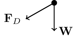
\[\begin{align} {\bf W} &= mg(-{\bf E}_y),\\ {\bf F}_D &= \underbrace{c_s \lnorm{\bf v}\rnorm}_{\text{magnitude}}\underbrace{\lp-\frac{{\bf v}}{\lnorm{\bf v}\rnorm}\rp}_{\text{unit direction}} = -c_s{\bf v}. \end{align}\] The Stokes drag (1851) applies at low speeds in viscous fluids.
Balance of linear momentum: \[\begin{align} {\bf F} &= \dot{\bf G},\\ -mg{\bf E}_y -c_s\lp\dot{x}{\bf E}_x+\dot{y}{\bf E}_y\rp &= m\lp\ddot{x}{\bf E}_x+\ddot{y}{\bf E}_y\rp. \end{align}\] Projecting: \[\begin{align} \lp{\bf F}=\dot{\bf G}\rp\cdot{\bf E}_x &\implies\quad -c_s\dot{x} = m\ddot{x}\\ \lp{\bf F}=\dot{\bf G}\rp\cdot{\bf E}_y &\implies\quad -mg-c_s\dot{y} = m\ddot{y} \end{align}\] Given initial conditions \(x_0, \dot{x}_0, y_0, \dot{y}_0\), these are an initial value problem (IVP).
Solving the \(x\)-equation (let \(v_x = \dot{x}\)): \[\begin{align} \lp{\bf F}=\dot{\bf G}\rp\cdot{\bf E}_x &\implies\quad -c_s\dot{x} = m\ddot{x},\\ \lp{\bf F}=\dot{\bf G}\rp\cdot{\bf E}_y &\implies\quad -mg-c_s\dot{y} = m\ddot{y}. \end{align}\] These equations give ODEs for \(x(t)\) and \(y(t)\). Given IC’s \(x_0, \dot{x}_0, y_0, \dot{y}_0\), we have an initial value problem (IVP).
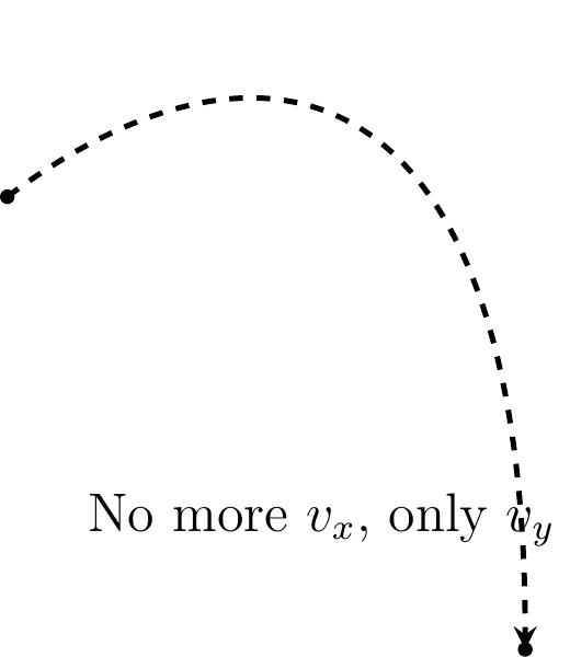
The \(x\)-equation is a first order ODE for \(v_x = \dot{x}\): \[\begin{align} \begin{split} -c_s v_x &= m\dot{v}_x\\ -\frac{c_s}{m}dt &= \frac{d v_x}{v_x}\\ -\frac{c_s}{m}\int_0^t d\tilde{t} &= \int_{v_{x_0}}^{v_c(t)}\frac{d\tilde{v}_x}{\tilde{v}_x}\\ -\frac{c_s}{m}t &= \ln\lp\frac{v_x}{v_{x_0}}\rp\\ v_x &= v_{x_0}e^{-\frac{c_s t}{m}} \end{split} \end{align}\] Note that \[\begin{align} \lim_{t\rightarrow\infty} v_x = 0. \end{align}\] Thus, the terminal velocity of the particle is only along \({\bf E}_y\).
Solving the \(y\)-equation: \[\begin{align} dt &= \frac{m dv_y}{-mg-c_s v_y}\\ \int_0^td\tilde{t} &= m\int_{v_{y_0}}^{v_y(t)}\frac{d\tilde{v}_y}{-mg-c_s\tilde{v}_y}\\ v_y &= -\frac{mg}{c_s}+\frac{1}{c_s}\lp mg+c_s v_{y_0}\rp e^{-c_st/m} \end{align}\] As \(t\rightarrow\infty\), \(v_y \rightarrow -\frac{mg}{c_s}\). Thus, the terminal velocity \[\begin{align} {\bf v}_{\text{term}} = \frac{mg}{c_s}\lp-{\bf E}_y\rp. \end{align}\] \[\begin{align} v_y = -\frac{mg}{c_s}+\frac{1}{c_s}\lp mg+c_s v_{y_0}\rp e^{-c_s t/m}. \end{align}\]
8.3.3 Example: Projectile Motion with Bluff Body Pressure Drag
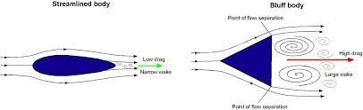
\[\begin{align} {\bf F}_D = \frac{1}{2}m C_D v^2\lp-\frac{\bf v}{\lnorm{\bf v}\rnorm}\rp, \end{align}\] where \(C_D\) is the drag coefficient, \(\rho\) is the density of the fluid, and \(A\) is the projected area in the direction of motion.
The equations of motion in this case (see primer section 1.6) need to be solved numerically. One way to do this is described in the video below.
8.4 Summary
Balance of linear momentum (BoLM / Newton’s 2nd law / Euler’s 1st law): \[\begin{align} \mathbf{F} = \dot{\mathbf{G}} = m\mathbf{a}. \end{align}\]
The four steps:
- Choose an origin; draw basis vectors; write and differentiate the position vector \(\mathbf{r}\).
- Draw the free body diagram; write expressions for all forces.
- Write the vector BoLM equation \(\sum\mathbf{F} = m\mathbf{a}\).
- Project along chosen directions and analyse to answer the question.
8.5 Exercises
The following problems are from Set 04 – Balance of Linear Momentum.
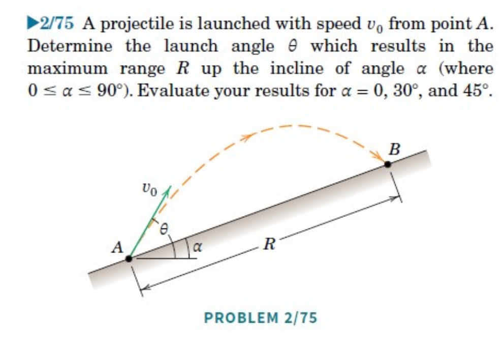
1. [MKB 2/75] Take \(\mathbf{E}_x\) along the incline and \(\mathbf{E}_y\) perpendicular to it (upwards); origin at \(A\). Follow the 4 steps. (ans. \(\theta = (90^\circ + \alpha)/2\))
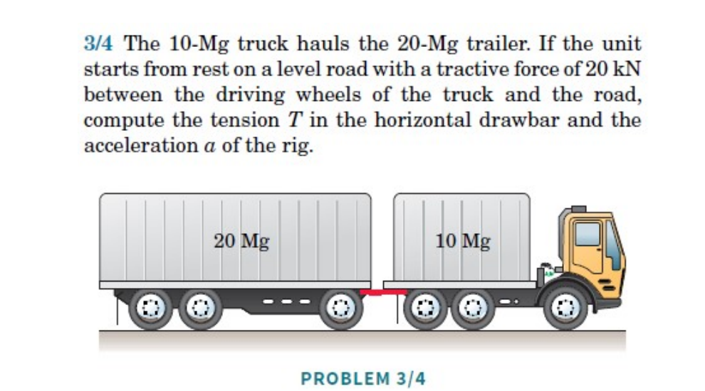
2. [MKB 3/004] Consider the whole truck system; follow the 4 steps to find the truck’s acceleration, then isolate a trailer to find the drawbar tension. (ans. \(T = 13.33\) kN, \(a = 0.667\) m/s\(^2\))
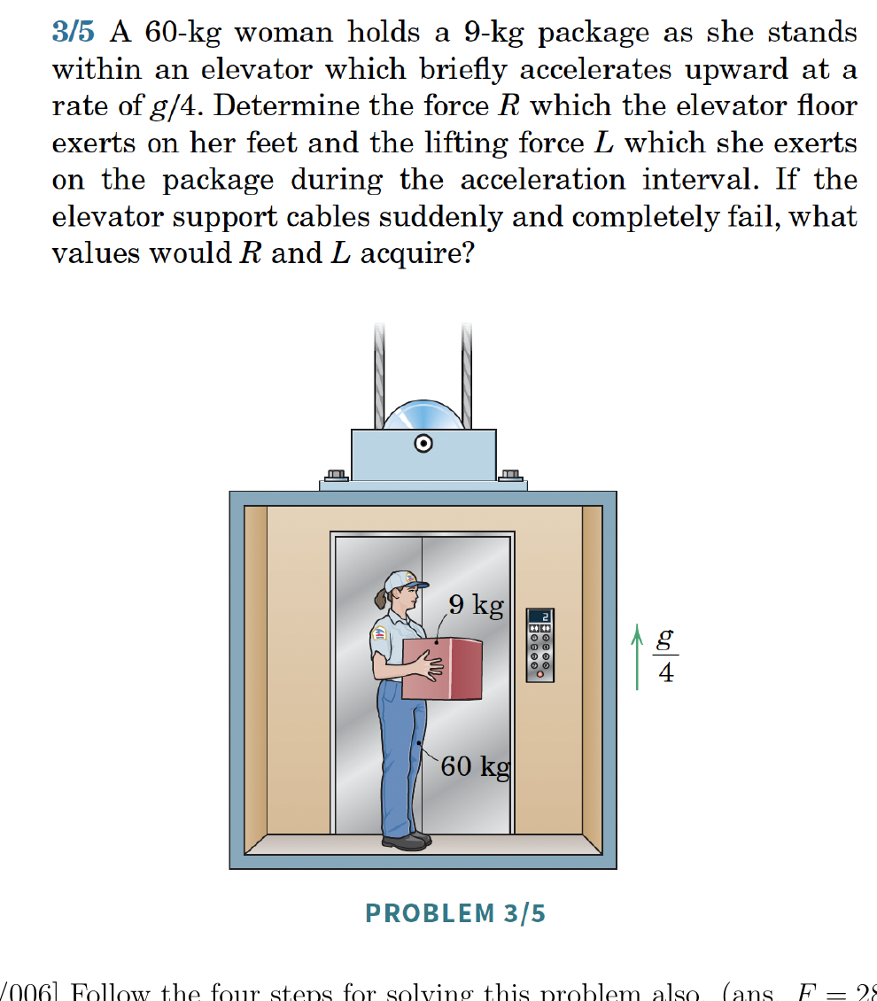
3. [MKB 3/005] For each part, determine your system and follow the 4 steps. (ans. \(R = 846\) N, \(L = 110.4\) N)
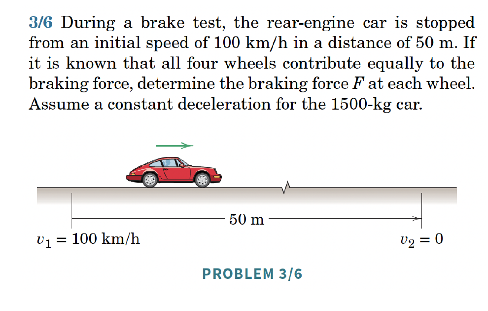
4. [MKB 3/006] Follow the four steps. (ans. \(F = 2890\) N)
5. [OOR Exercise 1.3]

6. [OOR Exercise 1.5]

7. [OOR Exercise 1.8]